

Architectures

Embedding

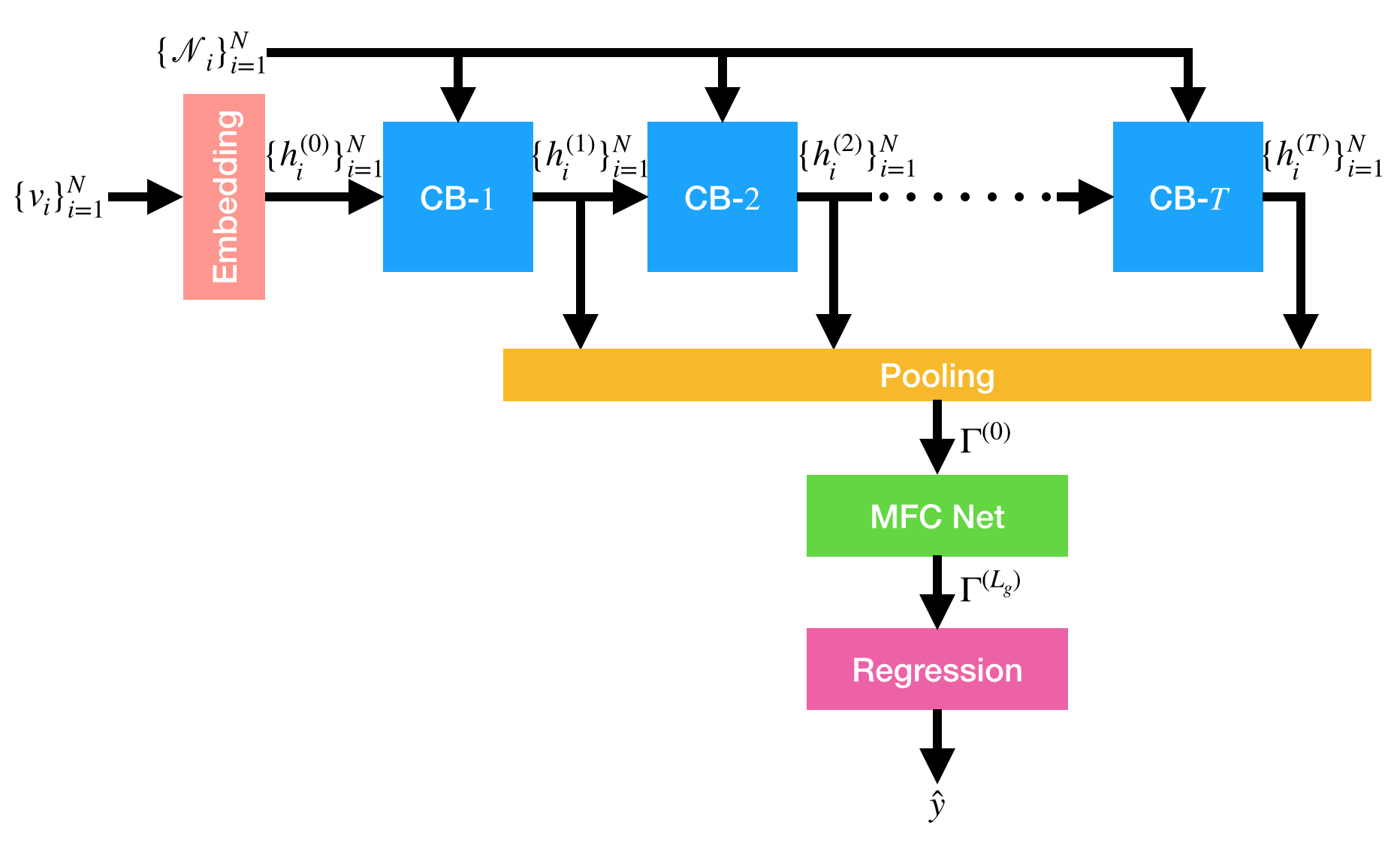
The $i$-th initial hidden state $h_{i}^{(0)} \in \mathbb{R}^{d_{h}}$ is given by the embedding of the $i$-th node state $v_{i}$ using the embedding matrix $E \in \mathbb{R}^{d_{v} \times d_{h}}$. The hidden states $\{ h_{i}^{(t)} \}_{t=1}^{T}$ are sequentially produced by stacked convolution blocks (CB), as shown in the figure of a CGNN architecture below.

Convolution Block

The CB is composed of an edge neural network (EdgeNet), a gated convolution layer, and a multi-layer fully connected neural network (MFCNet), as shown below.

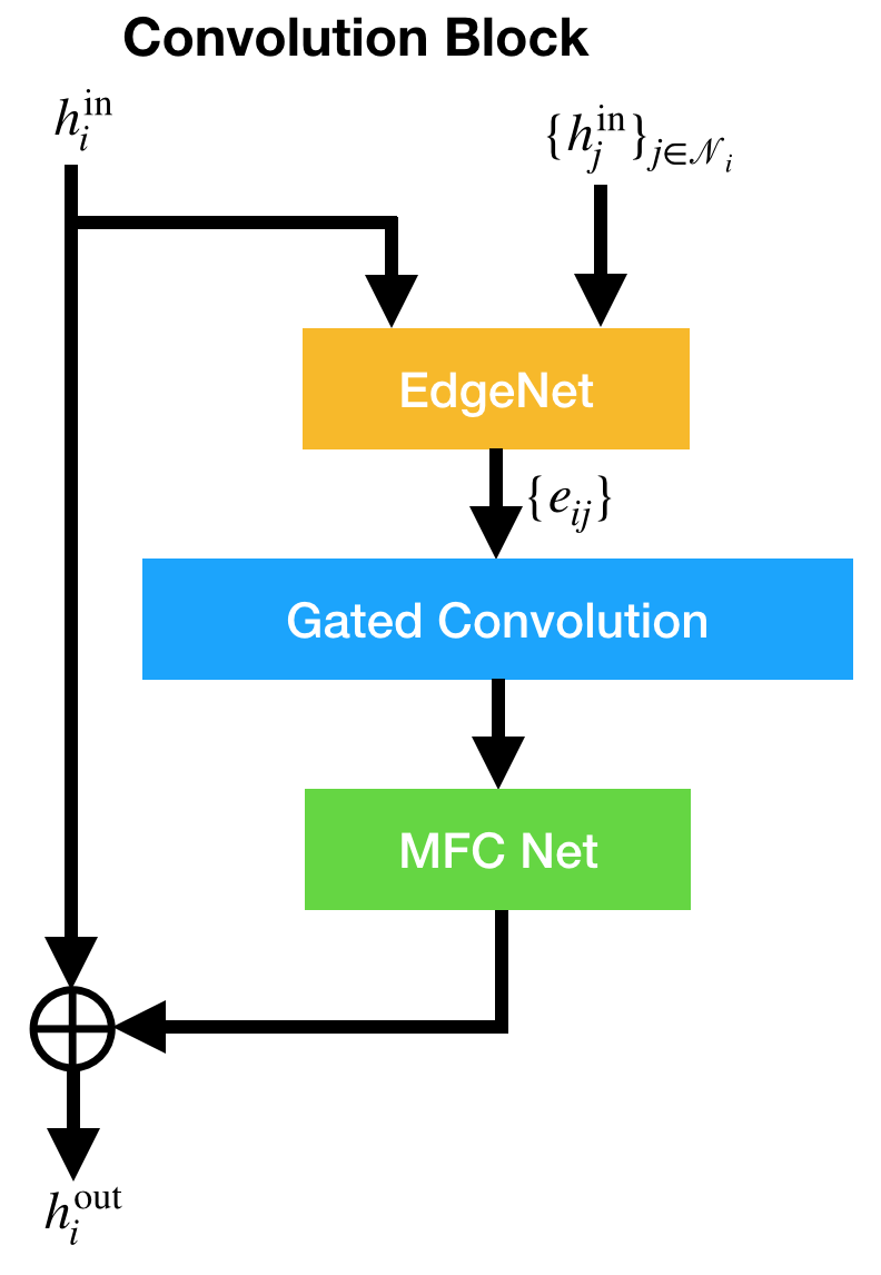
The EdgeNet produces edge states $e_{ij} \in \mathbb{R}^{d_{e}}$. The CB output $h_{i}^{\rm out}$ is the sum of the shortcut state $h_{i}^{\rm in}$ and the MFCNet output. The EdgeNet and MFCNet are optional components.

Multilayer Fully Connected Neural Networks

The MFCNet is composed of $L_{c}$ layers, each of which is given by

$$h^{\rm out} = f(h^{\rm in} W_{c}),$$

where $W_{c} \in \mathbb{R}^{d_{h} \times d_{h}}$ denotes a weight matrix, and $f(\cdot)$ denotes an activate function.

In neural network components presented below, $f(\cdot)$ appears repeatedly but is not needed to be the same activation function.

Gated Convolution

For $i$-th hidden state, given a sequence of vectors $\{ h_{j}^{\rm in} \}_{j \in \mathcal{N}_{i}}$, where $h_{j}^{\rm in} \in \mathbb{R}^{d_{c}}$ is either a hidden state ($d_{c}=d_{h}$) or an edge state ($d_{c}=d_{e}$), the CB outputs $h_{i}^{\rm out} \in \mathbb{R}^{d_{h}}$, as shown below.

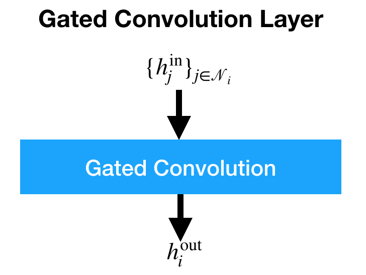
The $h_{i}^{\rm out}$ is given by

$$h_{i}^{\rm out} = \sum_{j \in {\cal N}_{i}} \sigma(h_{j}^{\rm in} W_{cg}) \odot f(h_{j}^{\rm in} W_{ch}),$$

where $W_{cg} \in \mathbb{R}^{d_{c} \times d_{h}}$ and $W_{ch} \in \mathbb{R}^{d_{c} \times d_{h}}$ denote weight matrices, $\sigma(\cdot)$ denotes the sigmoid function, and $\odot$ element-wise multiplication.

Edge Neural Networks

The EdgeNet is a multi-layer neural network composed of $L_{e}$ layers, as shown below.

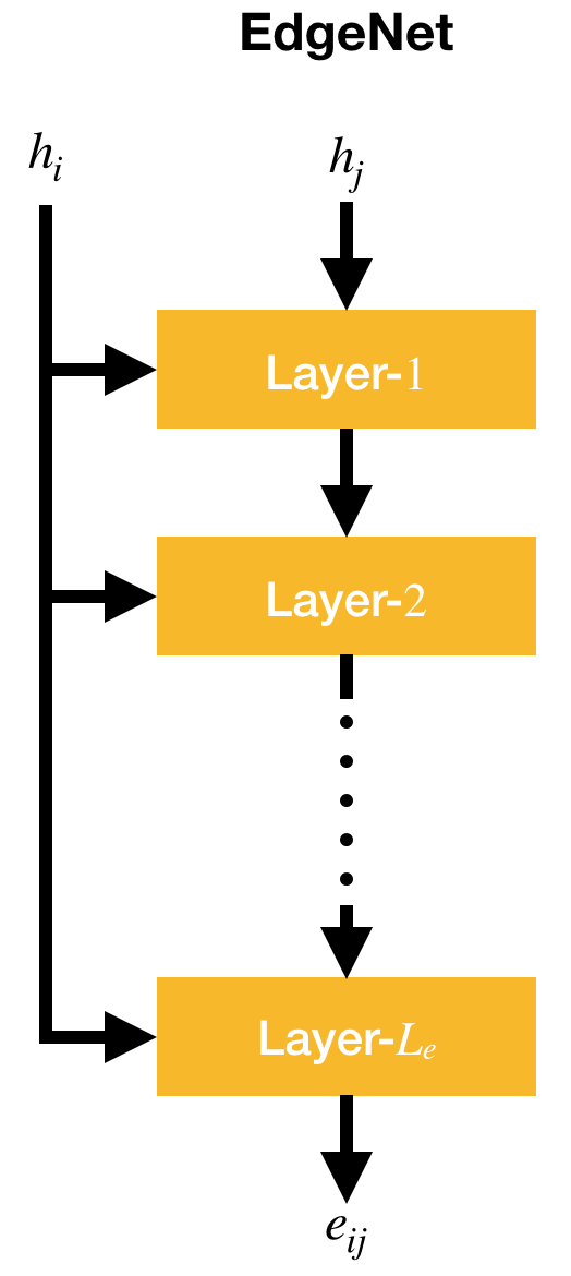
Given $i$-th hidden states $h_{i}$ and $j$-th hidden state $h_{j}$ where $j \in \mathcal{N}_{i}$, the EdgeNet outputs an edge state $e_{ij} \in \mathbb{R}^{d_{e}}$.

Three variants of the EdgeNet layer are presented below.

Original EdgeNet Layer

The EdgeNet layer first developed, as shown below, is made of a bilinear transformation.

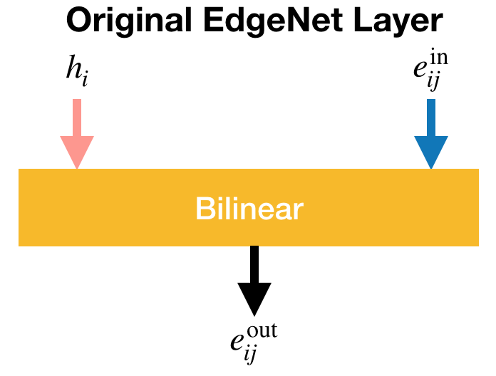
It is expressed as $$ e_{ij}^{\rm out} = f(\mathcal{B}(h_{i}, e_{ij}^{\rm in})), $$

and the bilinear transformation $\mathcal{B}(\cdot,\cdot)$ is defined by

$$\mathcal{B}(h, e) = h B e = \left\{ \sum_{p, q} h(p)B(p,q,r)e(q) \right\}_{r=1}^{d_{e}},$$

where $B$ is a weight tensor of order 3.

Fast EdgeNet Layer

The second EdgeNet layer is a fast version of $\mathcal{B}(\cdot,\cdot)$, and is composed of two fully connected layers and the element-wise multiplication, as shown below.

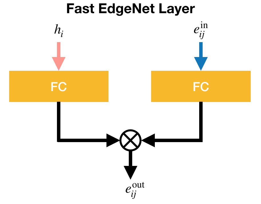
In the fast EdgeNet layer, the weight tensor is decomposed as

$$B(p,q,r) = W_{he}(p,r) W_{ee}(q,r),$$

where $W_{he}$ and $W_{ee}$ denote weight matrices. Then, this layer is expressed as

$$e_{ij}^{\rm out} = f((h_{i}W_{he}) \odot (e_{ij}^{\rm in}W_{ee})).$$

Moreover, the activation can be applied just after the two linear transformations, as expressed by

$$e_{ij}^{\rm out} = f(h_{i}W_{he}) \odot f(e_{ij}^{\rm in}W_{ee}).$$

Aggregate EdgeNet Layer

The last EdgeNet layer is based on aggregated transformations $\sum_{l=1}^{C} \mathcal{T}_{l}(h_{i}, e_{ij}^{\rm in})$, where $C$ is the cardinality, and $\mathcal{T}_{l}$ is a bilinear transformation block (BTB), as shown below.

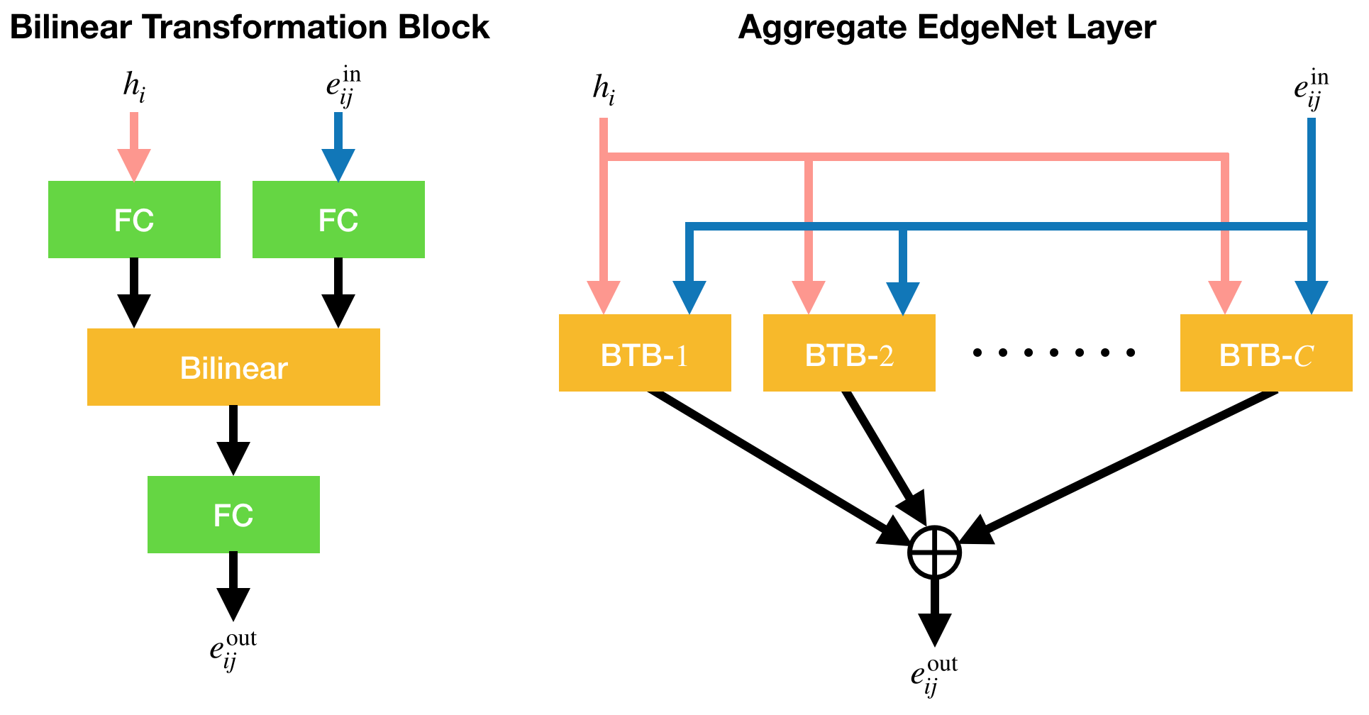
As shown in the left panel of the figure above, $\mathcal{T}_{l}$ is given by

$$e_{ij}^{\rm out} = \mathcal{B}_{l}(f(h_{i} W_{hb}), f(e_{ij}^{\rm in} W_{eb})) W_{be},$$

where $\mathcal{B}_{l}$ denotes a bilinear transformation $\mathbb{R}^{d_{b}} \times \mathbb{R}^{d_{b}} \to \mathbb{R}^{d_{b}}$ ($d_{b} \cdot C \approx d_{e}$ under normal use), and $W_{hb} \in \mathbb{R}^{d_{h} \times d_{b}}$, $W_{eb} \in \mathbb{R}^{d_{e} \times d_{b}}$, and $W_{be} \in \mathbb{R}^{d_{b} \times d_{e}}$ denote weight matrices.

As shown in the right panel, the aggregate EdgeNet layer outputs

$$e_{ij}^{\rm out} = f(\sum_{l=1}^{C} \mathcal{T}_{l}(h_{i}, e_{ij}^{\rm in})).$$

Edge Residual Neural Networks

The EdgeNet becomes a residual neural network when every EdgeNet layer is wrapped by the EdgeResNet layer, as shown below.

$$e_{ij}^{\rm out} = e_{ij}^{\rm in} W_{s} + \mathfrak{E}(h_{i}, e_{ij}^{\rm in}),$$

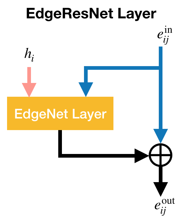
where $W_{s}$ denotes a weight matrix, and $\mathfrak{E}(\cdot, \cdot)$ an EdgeNet layer.

Pooling

The graph-level representation $\Gamma^{(0)} \in \mathbb{R}^{d_{h}}$ is made from all the hidden states $\{ h_{i}^{(t)} \}_{t=1,i=1}^{T,N}$ except for the initial ones. At each step $t$, the hidden states $\{ h_{i}^{(t)} \}_{i=1}^{N}$ are pooled with the gating mechanism as

$$\gamma_{t} = \frac{1}{N} \sum_{i=1}^{N} \sigma(h_{i}^{(t)} W_{\gamma}^{(t)} + b_{\gamma}^{(t)}) \odot h_{i}^{(t)},$$

where $W_{\gamma}^{(t)} \in \mathbb{R}^{d_{h} \times d_{h}}$ denotes a weight matrix, and $b_{\gamma}^{(t)} \in \mathbb{R}^{d_{h}}$ a bias vector. If the gating mechanism is not used, they are simply averaged as

$$\gamma_{t} = \frac{1}{N} \sum_{i=1}^{N} h_{i}^{(t)}.$$

Then, the graph-level states $\gamma_{1},\ldots,\gamma_{T}$ are weightedly averaged as

$$\Gamma^{(0)} = f(\sum_{t} \gamma_{t}W_{\Gamma}^{(t)}),$$

where $W_{\Gamma}^{(t)} \in \mathbb{R}^{d_{h} \times d_{h}}$ denotes a weight matrix. If only the final graph-level state $\gamma_{T}$ is used, it is simply activated as

$$\Gamma^{(0)} = f(\gamma_{T})$$

Graph-Level Neural Networks

The graph-level MFCNet is composed of $L_{g}$ layers, each of which outputs $\Gamma^{\rm out} \in \mathbb{R}^{d_{g}}$ given by

$$\Gamma^{\rm out} = f(\Gamma^{\rm in} W_{g} + b_{g}),$$

where $W_{g}$ denotes a weight matrix, and $b_{g} \in \mathbb{R}^{d_{g}}$ a bias vector. For the first layer $\Gamma^{\rm in} = \Gamma^{(0)}$ and $W_{g} \in \mathbb{R}^{d_{h} \times d_{g}}$ , and otherwise $\Gamma^{\rm in} \in \mathbb{R}^{d_{g}}$ and $W_{g} \in \mathbb{R}^{d_{g} \times d_{g}}$.

The final layer's output $\Gamma^{(L_{g})}$ is used as the input vector for the linear regression

$$\hat{y} = \Gamma^{(L_{g})} \cdot w_{r} + b_{r},$$

where $w_{r} \in \mathbb{R}^{d_{g}}$ denotes a weight vector, and $b_{r} \in \mathbb{R}$ a bias scalar.

Given true values $Y = \{ y_{i} \}_{i=1}^{N}$ and predicted values $\hat{Y} = \{ \hat{y}_{i} \}_{i=1}^{N}$, the mean squared error is calculated by

$$L(Y, \hat{Y}) = \frac{1}{N} \sum_{i=1}^{N} (y_i - \hat{y}_i)^{2},$$

which serves as the loss function for training a CGNN model. The mean absolute error (MAE) is also calculated by

$$\mathrm{MAE}(Y, \hat{Y}) = \frac{1}{N} \sum_{i=1}^{N} | y_i - \hat{y}_i |,$$

which is used as the validation metric to determine the best model in training. The root mean squared error $\sqrt{L(Y, \hat{Y})}$ is employed as an evaluation metric in testing as well as the MAE.